GENE Code Performance Overview

Caveats

• The following is based on the big-8 test case, with some modifcations. I believe what it shows is essentially typical behavior, but YMMV.
• I’m myself rather new to GENE, so I may have missed some things or gotten something wrong.
• I had some issue with the profiling of the CPU-only version, so the profile is not as detailed as it could be, but the important things are there.

Big picture

Most of the profiling I’m showing in the following is from a benchmark run on Summit that just used 4 CPU cores. The code is MPI parallelized. The profile on all procs should essentially looks the same, with maybe some minor imbalance at times due to physical boundary conditions.

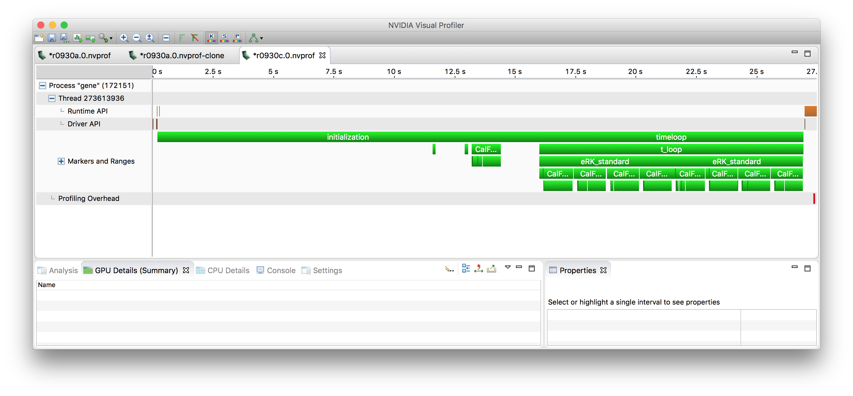
At the top level, you see two phases, initialization and timeloop. Since the initialization happens only once, its performance can be mostly ignored. The timeloop in this example is very short (only two time steps), but in real life wll be composed of a very large number of steps.

There can also be a phase 0, the autotuning. It is turned off in this run. That phase will determine parameters to get optimal performance, by

• evaluating different options for domain decomposition across the given number of MPI processes
• find an optimal parameter for cache blocking
• evaluate variants of various kernels which do the same operation but are implemented in some variations

As a general overview, the GENE code integrates 6-dimensional distribution functions in time, together with supporting lower-dimensional quantities like the electromagnetic field. Distribution functions are discretized in space (x, y, z), velocity space (v, w) and by species, The code often considers the distribution function arrays in a reshaped fashion, where it becomes f(i, j, klmn), ie. many i-j (x-y) slices, where klmn collapses the remaining 4 dims (k, l, m, n). This is what the cache blocking is based on. If nblocks == 1, all nk * nl * nm * nn slices are processed together. However, if nblocks > 1, nk * nl * nm * nn is subdivided into as many equal-sized pieces (“blocks”). Then, all operations are performed for just the first block, next all operations are performed on the second block, etc. In order to have a large amount of parallelism available for offloading onto the GPU, it is helpful to have large blocks, so in my work I have been using nblocks = 1, which for the test I’ve been using gives me a per-MPI process index space of 120 x 24 x 4 x 32 x 8 x 2 complex quanities, which is giving me pretty good results in terms of GPU performance already, but production runs are going to have yet larger problem sizes.

Timeloop

Zooming into the timeloop, once can see the general structure of time integration.

As stated above, in this benchmark case, the timeloop is only run for two steps, which show up as eRK_standard. Each timestep is performed by a 4th order Runge-Kutta (RK) method. which is comprised of 4 essentially identical stages. At each stage, the r.h.s. is calculated and then used to update some temporary fields, which eventually are combined into the new solution at time n+1.

In a real run, additionally, diagnostics will happen every so many time steps – this is ignored here.

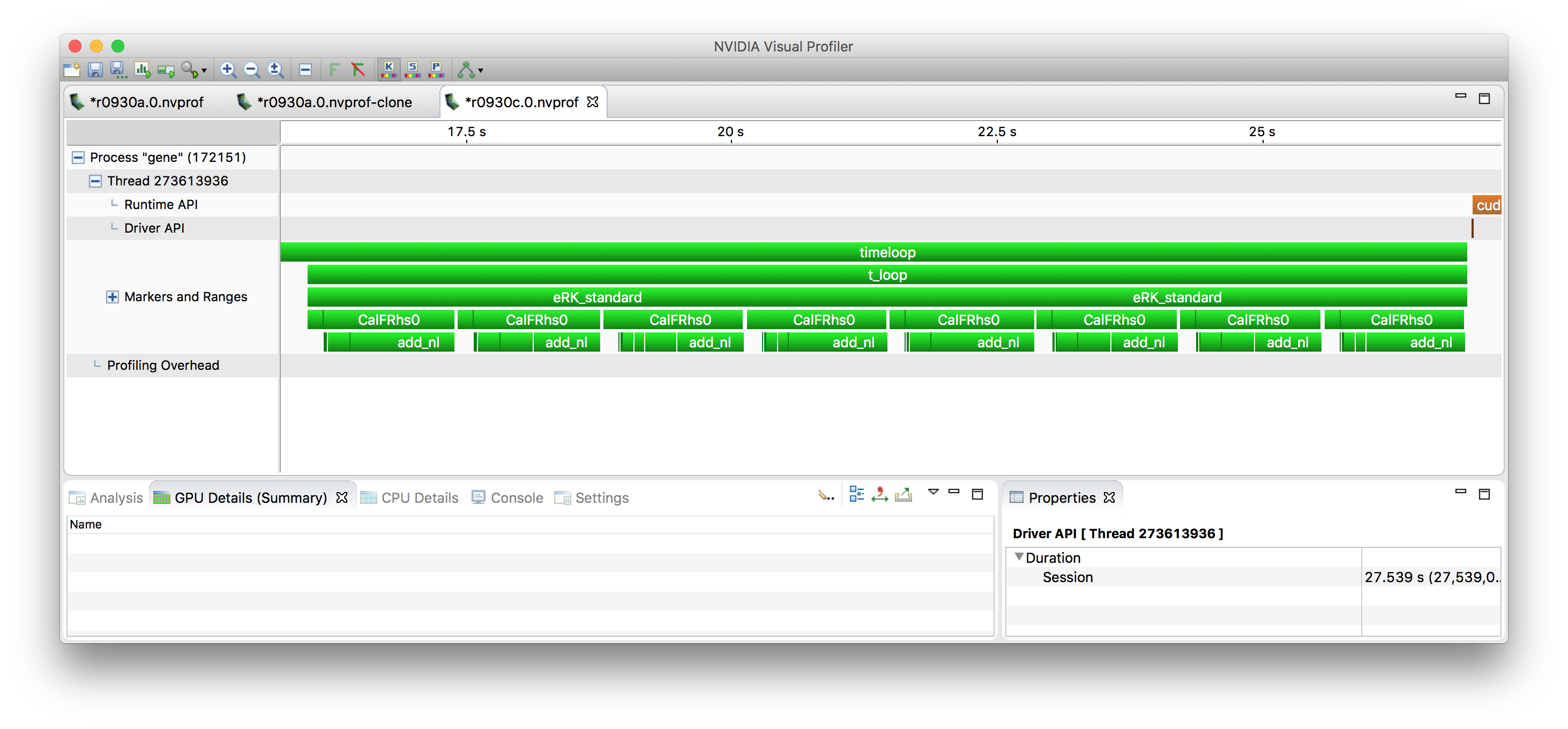
RK stage

Each RK stage consists of some prep work (calcaux) and then the computation of the r.h.s. (which is also a 6-d array, like the distribution functions) (‘’CalFRhs0’‘). At the end of the stage there are some updates of the temporary arrays, which is missing a marker in this profile, it’s in the white space after CalFRhs0.

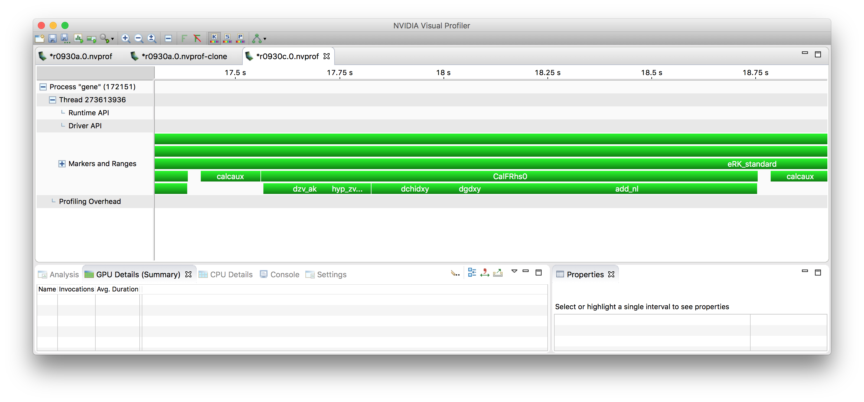
Computation of the r.h.s.

In the profile above, one can also see the steps involved in calculating the r.h.s. – essentially, terms from the physical equations are added up one after the other. These involve z and v derivatives (dzv_ak), hyperdiffusion (hyp_zv), various terms involving x and y derivatives (dfdxy (doesn’t show up separately), dchidxy, dgdxy), and then finally the nonlinear terms (add_nl).

One can see that while CalcFRhs0 if taken inclusively is where the majority of time is spent, it calls a number of other functions each of which take somewhat comparable amounts of time, so there is no one function that dominates the overall behavior.

The call chain doesn’t end here, functions like dchidxy are often further subdivided into a few actual computational kernels (typically I’d say about two or so).

The actual kernels are for the most part stencil computations – to show an example of a pretty large one:

do concurrent(n=bl(6):bu(6),&
  m=bl(5):bu(5), l=bl(4):bu(4), &
  k=bl(3):bu(3), j=bl(2):bu(2) )
b(i1:i2,j,k,l,m,n) = &
     sten(i1:i2, 1,k,l,m,n)*a(i1:i2,j,k  ,l-2,m,n) + &
     sten(i1:i2, 2,k,l,m,n)*a(i1:i2,j,k-1,l-1,m,n) + &
     sten(i1:i2, 3,k,l,m,n)*a(i1:i2,j,k  ,l-1,m,n) + &
     sten(i1:i2, 4,k,l,m,n)*a(i1:i2,j,k+1,l-1,m,n) + &
     sten(i1:i2, 5,k,l,m,n)*a(i1:i2,j,k-2,l  ,m,n) + &
     sten(i1:i2, 6,k,l,m,n)*a(i1:i2,j,k-1,l  ,m,n) + &
     sten(i1:i2, 7,k,l,m,n)*a(i1:i2,j,k  ,l  ,m,n) + &
     sten(i1:i2, 8,k,l,m,n)*a(i1:i2,j,k+1,l  ,m,n) + &
     sten(i1:i2, 9,k,l,m,n)*a(i1:i2,j,k+2,l  ,m,n) + &
     sten(i1:i2,10,k,l,m,n)*a(i1:i2,j,k-1,l+1,m,n) + &
     sten(i1:i2,11,k,l,m,n)*a(i1:i2,j,k  ,l+1,m,n) + &
     sten(i1:i2,12,k,l,m,n)*a(i1:i2,j,k+1,l+1,m,n) + &
     sten(i1:i2,13,k,l,m,n)*a(i1:i2,j,k  ,l+2,m,n)
 end do

The nonlinearity calculation is a bit different in that it involves FFTs into real space, then a number of stencil computations, then FFTs back. It consists of more kernels (maybe ~8) than the remaining terms, and the FFTs, so that’s why it shows up as slower.

The nonlinearity calculation as-is in Fortran is not well suited for offloading because it currently is written as slice-by-slice processing, rather than whole blocks, so the available parallelism is too small. (I have rewritten it by block for the CUDA work, but that’s in C++ – it wouldn’t be difficult to do this in Fortran, too, though.)

All the other stencil computations I think are decent candidates for offloading, they’re probably memory bound but can still can get pretty nice speed-ups.

There are some additional operations not covered in the above, for example the field solve (sparse linear algebra), and gyro-averaging (also linear algebra), but the vast majority of time is spent in various forms of stencil computations.

Current GPU work

So in order to make my point that off-loading works, let me show the current state of the GPU port using CUDA:

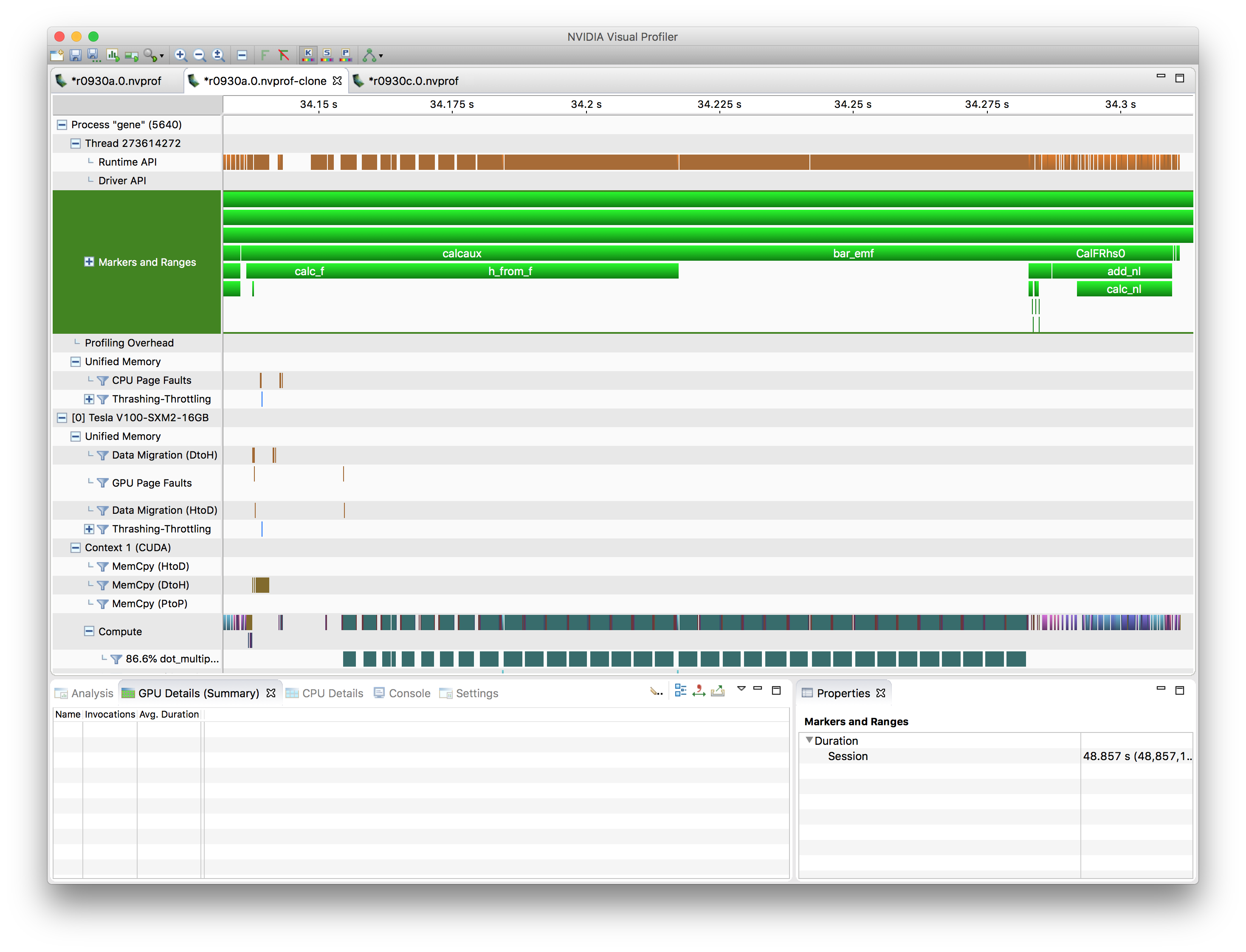
This profile also shows a single RK stage, ie., calcaux, bar_emf, and CalFRhs0. (bar_emf didn’t show up above since it’s pretty fast compared to its surrounding calcaux and bar_emf).

CalFRhs0 has been the focus of my work, and it’s vastly faster. It’s still comprised of the same underlying terms (too small to be labeled) and then the nonlinarity part. The nonlinearity part now takes a larger fraction of the r.h.s. calculation, but essentially, the picture is similar.

What’s different is that the intial part of the RK stage now takes a relatively larger fraction of time – the reason for this, I believe, is that the gyroaveraging, while on the GPU, calls way too many small kernels, so some refactoring into bigger kernels is needed there.

In terms of just looking at CalcFRhs0 itself, the timing went from 1.19 s (1 CPU core) to 27 ms (1 V100 GPU). This is of course an unfair comparison, but extrapolating given that Summit has 7 CPU cores / GPU, it’s a speed-up of 6.3x, which is at least a good start.